How Neural Networks Actually Learn

Without the Calculus (Mostly)

No prerequisites. Just curiosity.

The Hook: The Magic Trick You Use Every Day

Your phone unlocks the moment it sees your face. Google Photos finds “beach” pictures you never labeled. A self-driving car spots a pedestrian in the rain. Behind every one of these tricks is the same machine: a neural network that learned to see.

But here is the question that stops most students: how neural networks learn seems like it should require a mountain of terrifying math. Professors mention gradients, derivatives, the chain rule — and half the class quietly decides deep learning isn’t for them.

Here’s the honest answer: for CNN-style networks — the ones used in image recognition — most of what happens can be described using the linear algebra from our last blog. Vectors, matrices, dot products, transposes. Not all of it. But most. This post walks through the whole learning loop and shows you exactly where the one piece of calculus hides — and why you don’t need to master it to understand the picture.

What Is a Neural Network Actually Doing?

A convolutional neural network (CNN) has two jobs stacked on top of each other. One part pulls features out of an image. The other part turns those features into predictions. The feature-extraction happens in stages, and each stage builds on the one before it.

Early layers notice simple things. Edges. Corners. Sudden shifts from light to dark. Nothing impressive on its own. But the next layer takes those simple patterns and starts combining them into shapes. Go a few layers deeper, and the network is recognizing entire structures — wheels, eyes, whatever the training data happened to include. Simple to complex, one layer feeding the next.

The thing doing the actual pattern-detecting is called a kernel. And here’s the demystifying part: a kernel is a small matrix. That’s it. Nothing more behind the name.

The Building Blocks

1. Kernels — Sliding Matrices That Feel for Patterns

A kernel moves across an image a few pixels at a time. At each position it lands on, it performs a dot product between its own values and the pixel values underneath it — the same operation from the vectors section of the last blog, just repeated at every position the kernel passes over.

Real-world analogy: Imagine running your hand across a rough, textured surface in the dark. You can’t see the whole object, but you can still feel edges, bumps, and ridges. A kernel is doing something similar to a pixel grid. It doesn’t understand the whole image at once; it just detects small local patterns and passes that information along.

Here’s what makes CNNs special. Older image-processing techniques required someone to design these matrices by hand — one set of numbers for blurring, a different set for sharpening. A CNN skips that step. At first, a kernel is basically guessing; its numbers are random, so whatever it’s detecting isn’t useful yet. As training continues, those numbers shift gradually until the kernel starts responding to patterns that actually matter for the task. The network ends up discovering its own feature detectors instead of being handed them.

2. The Forward Pass — From Pixels to Prediction

An image is a grid of numbers — pixel brightness values in rows and columns. Exactly the kind of object linear algebra is built to handle.

The path from input to prediction follows the same pattern at every layer:

• Dot product: The kernel sits over a patch of pixels, multiplies its values against the pixels beneath it, and sums the result into one number.
• Bias: A bias term gets added on top, acting like a threshold — deciding how strong a signal needs to be before the neuron bothers reacting to it.
• Activation: The result passes through an activation function — usually ReLU, which zeroes anything negative, or Sigmoid, which squeezes the output into a range between 0 and 1.

Repeat this across every kernel and every layer, and a raw grid of pixel values slowly turns into a prediction — something like “87% chance this image contains a cat.” Every step along the way is a dot product followed by a threshold check. No calculus involved yet.

3. Non-Linearity — Why That Tiny Activation Step Matters So Much

This activation step is the only non-linear part of the whole process, and it’s doing more work than its size suggests. Without it, stacking multiple layers wouldn’t actually add anything — a chain of purely linear operations collapses into the equivalent of one layer, no matter how many you stack. Non-linearity is what keeps depth meaningful.

Real-world analogy: Think of mixing paint. If you’re only allowed to mix shades of gray, then no matter how many mixing steps you chain together, you still end up with gray — a hundred steps achieve nothing a single step couldn’t. The activation function is like being allowed to add a drop of color between steps. Suddenly each layer can produce something genuinely new.

4. Loss — Measuring How Wrong the Network Is

Kernels start out random, so an untrained network’s early predictions tend to be bad. The gap between what it predicted and what the correct answer actually was is called the loss. Training exists to shrink that gap.

Real-world analogy: Loss is like the score in golf — lower is better, zero is perfect, and every training step is one careful swing trying to bring the number down.

5. Backpropagation — Sending the Blame Backward

Here’s the catch: the loss is only measurable at the output layer. So how does a kernel sitting near the input, several layers removed from the output, know what to adjust?

The error gets sent backward through the network, layer by layer, starting at the output and working toward the input — which is where the name backpropagation actually comes from. Each layer works out how much it contributed to the overall error, and it does this using the same weight matrices from the forward pass, now applied in transposed form. Forward pass pushes data forward through the matrices; backward pass pushes error backward through the transposed ones. The same transpose covered in the last blog.

Once a layer’s share of the blame is worked out, its kernel weights shift slightly in the direction that reduces it. How big that shift is depends on the learning rate — too large and training overshoots and bounces around; too small and it crawls. A full pass through the training data is an epoch, and batch size is just how many samples get processed before the weights update. Naming conventions, not new math.

Okay, So Where Does the Calculus Actually Hide?

Honesty time. Describing backprop as “just applying the matrices in transposed form” is a simplification. The actual mechanism computing how much each weight is to blame relies on the chain rule — which is calculus — working layer by layer through the activation functions along the way. The transpose is a real and important part of the picture; it’s what makes the backward pass computationally efficient. But it isn’t the whole mechanism on its own.

Here’s the framing that matters: the calculus lives in that one step — figuring out exactly how much each kernel is to blame for the final error. But the output of that step is a vector, an object that fits neatly into the same linear algebra picture as everything else here. It points in the direction that increases the loss, and the network moves its weights the opposite way. Calculus produces the input to that step. Everything after it — the actual movement through the network — is linear algebra.

🌱   🌱   🌱

A Concrete Example: One Kernel Detecting One Edge

Let’s do the actual math for a single kernel at a single position — the same way we rotated a point in the last blog. Don’t worry, it’s just multiplication and addition.

Suppose the kernel is sitting over this 3×3 patch of an image. Low numbers are dark pixels, high numbers are bright — so this patch is dark on the left and bright on the right. In other words, there’s a vertical edge here:

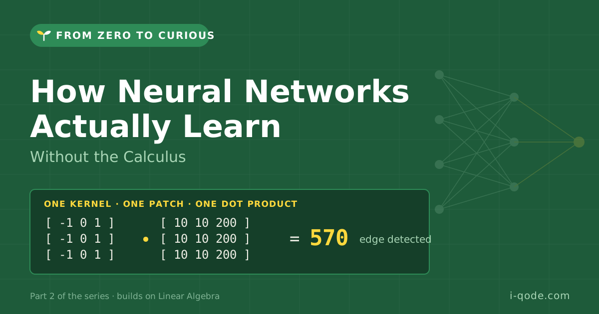
Patch P =  [ 10  10  200 ]
           [ 10  10  200 ]
           [ 10  10  200 ]

And here’s a classic vertical-edge-detecting kernel — negative on the left, positive on the right:

Kernel K = [ -1   0   1 ]
           [ -1   0   1 ]
           [ -1   0   1 ]

The dot product: multiply each pair of matching positions, then add everything up.

Row 1:  (-1)(10) + (0)(10) + (1)(200)  =  190
Row 2:  (-1)(10) + (0)(10) + (1)(200)  =  190
Row 3:  (-1)(10) + (0)(10) + (1)(200)  =  190

Total  =  570   →  strong response: EDGE DETECTED

Now slide the same kernel onto a boring, uniform patch where every pixel is 10. Each row gives (−10 + 0 + 10) = 0, so the total is 0 — no response, no edge. That’s the entire trick: big number means “my pattern is here,” zero means “nothing to see.” A CNN does this millions of times per image, with hundreds of kernels, at every position — and every single one of those operations is a dot product.

Your Learning Roadmap

Want to go from understanding neural networks to actually building one? Here’s the path, in order.

Step 1 — Watch It Happen Visually

3Blue1Brown’s “Neural Networks” series on YouTube is the single best visual introduction ever made. Four videos, zero prerequisites beyond what you’ve read here. Watch it before touching any code.

Step 2 — Play Before You Build

Open TensorFlow Playground (playground.tensorflow.org) in your browser. It’s a neural network you can train by clicking — watch layers learn patterns in real time, break it, fix it, develop intuition with zero setup.

Step 3 — Build a Tiny One From Scratch

Using Python and NumPy — no frameworks — write a small network that learns something simple, like recognizing handwritten digits from the MNIST dataset. It will hurt a little. That’s the point. You’ll understand forward passes and weight updates forever afterward.

Step 4 — Graduate to PyTorch

Once the from-scratch version works, rebuild it in PyTorch in a tenth of the code. Now you’re using the same tool as every AI lab on the planet, and you actually understand what it’s doing under the hood — which most people using it don’t.

💡 Looking for real-world experience? Companies like i-Qode Digital Solutions are constantly looking for students who understand what’s inside the black box — not just how to call an API. A from-scratch neural network in your portfolio says more to an interviewer than a dozen certificates.

Wrapping Up

Strip away the intimidating vocabulary, and a convolutional neural network is a surprisingly honest machine. Kernels are small matrices. The forward pass is a repeated dot product followed by a threshold and an activation function. Backpropagation reuses the forward pass’s weight matrices in transposed form to move error backward through the network, with the chain rule doing the underlying work of figuring out exact contributions.

None of this needed new mathematical tools beyond what the last post introduced. Matrices and vectors, applied over and over, adjusted a small amount at a time. That’s how neural networks learn.

So the next time your phone recognizes your face in the dark, you’ll know: that’s not magic. That’s a few hundred small matrices that spent weeks practicing.

🌱

That’s it for this edition of From Zero to Curious.
You started at zero. Hopefully, you’re leaving curious.

References & Further Reading

• From Zero to Curious: Linear Algebra — The Hidden Engine of CS and AI (start here if you haven’t read Part 1)
• 3Blue1Brown — Neural Networks (YouTube series)
• TensorFlow Playground — train a neural network in your browser
• Michael Nielsen — Neural Networks and Deep Learning (free online book)
• Deep Learning by Goodfellow, Bengio, and Courville — Chapters 6 & 9
• PyTorch tutorials — for hands-on practice